python でパワースペクトルを計算する方法

matplotlib と scipy で FFT を計算する方法

matplotlib と scipy のどちらもパワースペクトルを計算する方法があるが、両者でデフォルトで持っている関数と定義が違う。大概の使い分けは次の通り。

単純にパワースペクトルを計算する場合、mlab.psd が一番簡単。
scipy.fftpack を使うと実部と虚部が得られる。位相の計算など細かいことが可能だか、規格化は自分で行う必要あり。

どちらでやっても、パーセバルの定理から全パワーは同じになるが、両者の規格化の違いを考えないとパワースペクトルの縦軸が完璧に同じにならない。

ここでは単純な三角関数を両方の方法でフーリエ変換して、完璧にmatplotlibとscipyのFFTで結果が同じになる例を示す。おまけで、パワースペクトルから三角波の振幅を求めて、それがもとの三角関数の振幅と同じになること、フィルターを入れるとどういう影響があるかを紹介する。

問題設定

フーリエ変換する前の関数

縦軸は特に意味はないが、電圧V(t)という信号で単一の三角関数を考える。最も簡単な表式として$$y=V(t)=\sin(t)$$を用いる。周期 $f$ の三角関数は、$$\sin(2\pi ft)$$と書けるので、周期 $$f=1/2\pi$$ という設定になる。振幅は1.0である。

これを mlab.psdとscipy.fftpackの両方でフーリエ変換してパワーを計算する。それぞれ、hanning filter をかけた場合も計算し、違いを見てみる。

時間分解能 dt は0.1秒とする。ナイキスト周波数 f_n は、その逆数の半分で、5Hzとなる。

サンプルコード

qiita_fft_matplotlib_scipy_comp.py

#!/usr/bin/env python

"""
#2013-03-12 ; ver 1.0; First version, using Sawada-kun's code
#2013-08-28 ; ver 1.1; refactoring
#2020-03-31 ; ver 1.2; updated for python3
"""
__version__=  '1.2'

import numpy as np
import scipy as sp
import scipy.fftpack as sf
import matplotlib.mlab as mlab
import matplotlib.pyplot as plt
import optparse

def scipy_fft(inputarray,dt,filtname=None, pltfrag=False):

    bin = len(inputarray)
    if filtname == None:
        filt = np.ones(len(inputarray))
    elif filtname == 'hanning':
#        filt = sp.hanning(len(inputarray))
        filt = np.hanning(len(inputarray))                
    else:
        print('No support for filtname=%s' % filtname)
        exit()

    freq = sf.fftfreq(bin,dt)[0:int(bin/2)]
    df = freq[1]-freq[0]
    fft = sf.fft(inputarray*filt,bin)[0:int(bin/2)]

    real = fft.real
    imag = fft.imag
    psd = np.abs(fft)/np.sqrt(df)/(bin/np.sqrt(2.))

    if pltfrag: 
        binarray = range(0,bin,1)
        F = plt.figure(figsize=(10,8.))
        plt.subplots_adjust(wspace = 0.1, hspace = 0.3, top=0.9, bottom = 0.08, right=0.92, left = 0.1)
        ax = plt.subplot(1,1,1)
        plt.title("check fft of scipy")
        plt.xscale('linear')
        plt.grid(True)
        plt.xlabel(r'number of bins')
        plt.ylabel('FFT input')
        plt.errorbar(binarray, inputarray, fmt='r', label="raw data")
        plt.errorbar(binarray, filt, fmt='b--', label="filter")
        plt.errorbar(binarray, inputarray * filt, fmt='g', label="filtered raw data")
        plt.legend(numpoints=1, frameon=False, loc=1)
        plt.savefig("scipy_rawdata_beforefft.png")
        plt.show()

    return(freq,real,imag,psd)


usage = u'%prog [-t 100] [-d TRUE]'
version = __version__
parser = optparse.OptionParser(usage=usage, version=version)
parser.add_option('-f', '--outputfilename', action='store',type='string',help='output name',metavar='OUTPUTFILENAME', default='normcheck')
parser.add_option('-d', '--debug', action='store_true', help='The flag to show detailed information', metavar='DEBUG', default=False)
parser.add_option('-t', '--timelength', action='store', type='float', help='Time length of input data', metavar='TIMELENGTH', default=20.)
options, args = parser.parse_args()
argc = len(args)

outputfilename =  options.outputfilename
debug =  options.debug
timelength =  options.timelength

timebin = 0.1 # timing resolution
# Define Sine curve
inputf = 1/ (2 * np.pi) # f = 1/2pi -> sin (t)
inputt = 1 / inputf # T = 1/f 
t = np.arange(0.0, timelength*np.pi, timebin)
c = np.sin(t)
fNum = len(c)
Nyquist = 0.5 / timebin
Fbin = Nyquist / (0.5 * fNum)
fftnorm =  1. / (np.sqrt(2) * np.sqrt(Fbin))

print("................. Time domain ................................")   
print("timebin = " + str(timebin) + " (sec) ")
print("frequency = " + str(inputf) + " (Hz) ")
print("period = " + str(inputt) + " (s) ")
print("Nyquist (Hz) = " + str(Nyquist) + " (Hz) ")
print("Frequency bin size (Hz) = " + str(Fbin) + " (Hz) ")
print("FFT norm  = " + str(fftnorm) + "\n")

# Do FFT.
# Hanning Filtered
psd2, freqlist = mlab.psd(c,
                         fNum,
                         1./timebin,
                         window=mlab.window_hanning,
                         sides='onesided',
                         scale_by_freq=True
                         )
psd = np.sqrt(psd2)    

spfreq,spreal,spimag,sppower = scipy_fft(c,timebin,'hanning',True)

# No Filter
psd2_nofil, freqlist_nofil = mlab.psd(c,
                                     fNum,
                                     1./timebin,
                                     window=mlab.window_none,
                                     sides='onesided',
                                     scale_by_freq=True
                                     )
psd_nofil = np.sqrt(psd2_nofil)    
spfreq_nf,spreal_nf,spimag_nf,sppower_nf = scipy_fft(c,timebin,None)

# Get input norm from FFT intergral
print("................. FFT results ................................")       
amp = np.sqrt(2) * np.sqrt(np.sum(psd * psd) * Fbin)
print("Amp  = " + str(amp))
peakval = amp / (np.sqrt(2) * np.sqrt(Fbin) )
print("Peakval  = " + str(peakval))

# (1) Plot Time vs. Raw value
F = plt.figure(figsize=(10,8.))
plt.subplots_adjust(wspace = 0.1, hspace = 0.3, top=0.9, bottom = 0.08, right=0.92, left = 0.1)

ax = plt.subplot(3,1,1)
plt.title("FFT Norm Check")
plt.xscale('linear')
plt.xlabel(r'Time (s)')
plt.ylabel('FFT input (V)')
plt.errorbar(t, c, fmt='r', label="raw data")
plt.errorbar(t, amp * np.ones(len(c)), fmt='b--', label="Amplitude from FFT", alpha=0.5, lw=1)
plt.ylim(-2,2)
plt.legend(numpoints=1, frameon=True, loc="best", fontsize=8)

# (2a) Plot Freq vs. Power (log-log)
ax = plt.subplot(3,1,2)
plt.xscale('log')
plt.yscale('log')
plt.xlabel(r'Frequency (Hz)')
plt.ylabel(r'FFT Output (V/$\sqrt{Hz}$)')
plt.errorbar(freqlist_nofil , psd_nofil, fmt='r-', label="Window None, matplotlib", alpha=0.8)    
plt.errorbar(freqlist, psd, fmt='b-', label="Window Hanning, matplotlib", alpha=0.8)
plt.errorbar(spfreq_nf, sppower_nf, fmt='mo', label="Window None, scipy", ms = 3, alpha=0.8)    
plt.errorbar(spfreq, sppower, fmt='co', label="Window Hanning, scipy", ms = 3, alpha=0.8)
plt.errorbar(freqlist, fftnorm * np.ones(len(freqlist)), fmt='r--', label=r"1./($\sqrt{2} \sqrt{Fbin}$)", alpha=0.5, lw=1)
plt.legend(numpoints=1, frameon=True, loc="best", fontsize=8)

# (2b) Plot Freq vs. Power (lin-lin)
ax = plt.subplot(3,1,3)
plt.xscale('linear')
plt.xlim(0.1,0.2)
plt.yscale('linear')
plt.xlabel(r'Frequency (Hz)')
plt.ylabel(r'FFT Output (V/$\sqrt{Hz}$)')    
plt.errorbar(freqlist_nofil , psd_nofil, fmt='r-', label="Window None, matplotlib", alpha=0.8)    
plt.errorbar(freqlist, psd, fmt='b-', label="Window Hanning, matplotlib", alpha=0.8)
plt.errorbar(spfreq_nf, sppower_nf, fmt='mo', label="Window None, scipy", ms = 3, alpha=0.8)    
plt.errorbar(spfreq, sppower, fmt='co', label="Window Hanning, scipy", ms = 3, alpha=0.8)
plt.errorbar(freqlist, fftnorm * np.ones(len(freqlist)), fmt='r--', label=r"1./($\sqrt{2} \sqrt{Fbin}$)", alpha=0.5, lw=1)
plt.legend(numpoints=1, frameon=True, loc="best", fontsize=8)

plt.savefig("fft_norm_check.png")
plt.show()

実行方法は、単に何も指定しないか、-t で時間幅を変えるくらい。

$ python qiita_fft_matplotlib_scipy_comp.py -h
Usage: qiita_fft_matplotlib_scipy_comp.py [-t 100] [-d TRUE]

Options:
  --version             show program's version number and exit
  -h, --help            show this help message and exit
  -f OUTPUTFILENAME, --outputfilename=OUTPUTFILENAME
                        output name
  -d, --debug           The flag to show detailed information
  -t TIMELENGTH, --timelength=TIMELENGTH
                        Time length of input data

フーリエ変換する前の時系列データ

何もオプションを指定しないで実行すると、次のような時系列データのフーリエ変換を実行する。

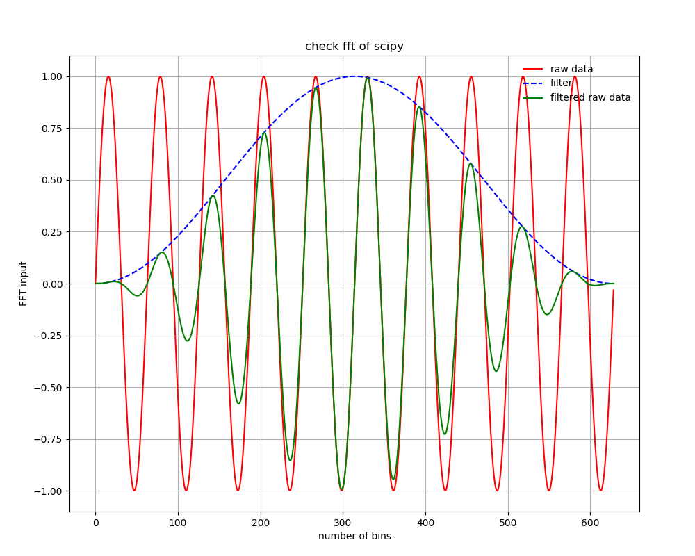
hanningフィルタがかかる場合、元の時系列データ(赤)に対して、hanning フィルタ(青)がかかって、緑のデータをフーリエ変換することになる。フィルターを使わない場合は、赤を周期境界条件でフーリエ変換することになる。フィルターをかける場合は、オフセット(周波数=0の成分)が乗っている場合は、フィルターによる人為的な低周波ノイズがのる場合があるので、フィルターを使う場合はDC成分は引いてから使うほうがよい。

パワースペクトルの計算結果

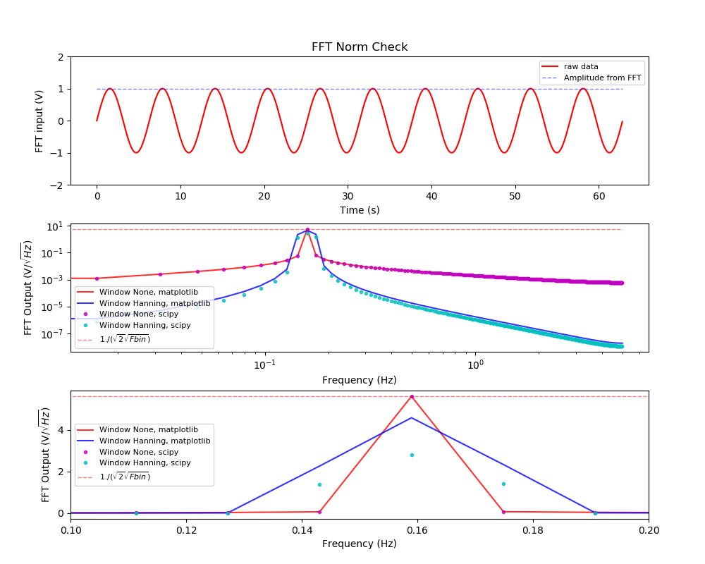
(上段) フーリエ変換する時系列データ。パワースペクトルから計算した時系列データの振幅を重ねて表示した。(中段)赤がフィルターなしの場合、青がhanning filter ありの場合。実線がmatplotlibで計算した場合で、ドットはscipyで計算したもの。赤い薄い線は時系列データから推定したパワーの値。(下段)中段の縦軸リニアバージョン。

パーセバルの定理の確認

パーセバルの定理より、周波数空間と時空間の積分値のパワーは一致する。三角関数の場合は、変動のパワー(RMS)と振幅は$\sqrt{2}$で結ばれているので、振幅とRMSは相互に変換できる。ここでは、周波数空間を全積分したパワーから時系列データの振幅(この例では1)を計算し、それが一致することを上の絵の青点線で示した。

周波数空間で積分している箇所は、コードの、

amp = np.sqrt(2) * np.sqrt(np.sum(psd * psd) * Fbin)
print("Amp  = " + str(amp))

に該当する。

amplitude = \sqrt{2} \sqrt{ \sum_i psd(f_i)^2 \Delta f }

で計算している。この値がこの例では1になっていて、

plt.errorbar(t, amp * np.ones(len(c)), fmt='b--', label="Amplitude from FFT", alpha=0.5, lw=1)

で上段に青い点線でプロットしている。

hanning フィルターの効果

フィルタがなければ、mlab.psdとscipy.fftpack は完璧に一致する。hanning filterを使うとパワーはある割合で下がるのでその分を補正する必要があるのだが、matplotlibとscipyで定義が違うのか(深追いしてない)、デフォルトのまま使うと両者の結果は一致はしない。

コードの補足

mlab.psdの使い方

# Do FFT.
# Hanning Filtered
psd2, freqlist = mlab.psd(c,
                         fNum,
                         1./timebin,
                         window=mlab.window_hanning,
                         sides='onesided',
                         scale_by_freq=True
                         )
psd = np.sqrt(psd2)

ここで、c はFFTしたい同時間感覚幅で取得されたデータ。FFTはサンプルが全く同じ時間間隔でされたことを前提としている。(もし、時間間隔が変わる場合にはダイレクトに離散フーリエ変換をするが、計算時間はかかる。精密な実験などではそうする場合もある。) fNumはサンプル数、1/timebin で時間幅の逆数を指定する、window は None とすれば何もなし、mlabのオプションにいろんなフィルターがあるが、ここでは hanningの例を示した。sidesは onesided で片面(周波数が正の値)で積分したときにトータルのパワーが時系列のパワーと一致するように規格化するという意味。scale_by_freq で、周波数あたりに直す。これにより、返り値はpower^2/Hzの単位となる。ここでは最後に、psd = np.sqrt(psd2) をすることで、power/sqrt(Hz)の単位にしている。

scipy.fftpack の使い方

    freq = sf.fftfreq(bin,dt)[0:int(bin/2)]
    df = freq[1]-freq[0]
    fft = sf.fft(inputarray*filt,bin)[0:int(bin/2)]

fftfreq という関数を使うことで、周波数を計算してくれる。これは実はとっても大事な機能である。なぜかというと、ここscipyのfftでは複素フーリエ変換を実行するのであるが、返り値は実部と虚部の係数であり、それをどういう周波数の順番でユーザーに返すのかは自明ではないので、対応のとれた周波数を返してくれる関数が必要になる。

    real = fft.real
    imag = fft.imag
    psd = np.abs(fft)/np.sqrt(df)/(bin/np.sqrt(2.))

で、実部を虚部を取り出し、片側(周波数が正)で規格化して帳尻があるように規格化を行う。

matplotlibとscipyのフーリエ変換(FFT)を用いてパーシバルの定理を確認する方法