第二回目です。
前回と同様にInstant Gratificationのコンペでchris Deotteさんの二個目のアプローチ。
今回もカーネルとコードを紹介する。
早速
SVMではスコア0.925を出すことができた。
前回のロジスティック回帰では単純な線形モデルmagic変数ごとにを使った。
今回は非線形のSVMを使い、4次の多項式モデルを作成した。
モデルは、特徴量選択を分散の閾値で判断した。
モデルは256の変数があるが、分散閾値により40個ほどまで減らした。(この40はモデルごとに違う)
wheezy・・・magicという変数が質的データであり、他の変数と特別な関係を持っている。
import numpy as np, pandas as pd, os
from sklearn.linear_model import LogisticRegression
from sklearn.model_selection import StratifiedKFold
from sklearn.metrics import roc_auc_score

train = pd.read_csv('train.csv')
test = pd.read_csv('test.csv')

train.head()
データは前回の記事かカーネルを参考にしていただきたい。
# LOAD LIBRARIES
from sklearn.svm import SVC
from sklearn.feature_selection import VarianceThreshold
from sklearn.model_selection import StratifiedKFold
from sklearn.metrics import roc_auc_score

# INITIALIZE VARIABLES
oof = np.zeros(len(train))
preds = np.zeros(len(test))
cols = [c for c in train.columns if c not in ['id', 'target', 'wheezy-copper-turtle-magic']]
trainからidとtargetとカテゴリカルデータを取り除いている。
以下でモデル作成をしているが、コードの中身の意味はコード中にコメントアウトで書き込む。
# BUILD 512 SEPARATE NON-LINEAR MODELS
for i in range(512):

    # EXTRACT SUBSET OF DATASET WHERE WHEEZY-MAGIC EQUALS I
    train2 = train[train['wheezy-copper-turtle-magic']==i]
    test2 = test[test['wheezy-copper-turtle-magic']==i]
    idx1 = train2.index; idx2 = test2.index
    train2.reset_index(drop=True,inplace=True)

    #カテゴリカルデータであるwheezyは0~512の数字?になっている。
    #カテゴリカルが1の時、ほかの変数はどうなってますか?
    #ほかのカラムを調べる。そのインデックスを取ってきてる。
    #だいたいカテゴリカル1つに対して500行くらいのデータが取れる。

    # FEATURE SELECTION (USE APPROX 40 OF 255 FEATURES)
    sel = VarianceThreshold(threshold=1.5).fit(train2[cols])
    train3 = sel.transform(train2[cols])
    test3 = sel.transform(test2[cols])

    # STRATIFIED K FOLD (Using splits=25 scores 0.002 better but is slower)
    #データを25分割したら少しだけ精度が上がったけど、すっごい時間かかったからやめるね。
    skf = StratifiedKFold(n_splits=11, random_state=42)
    for train_index, test_index in skf.split(train3, train2['target']):

        # MODEL WITH SUPPORT VECTOR MACHINE
        clf = SVC(probability=True,kernel='poly',degree=4,gamma='auto')
        clf.fit(train3[train_index,:],train2.loc[train_index]['target'])
        oof[idx1[test_index]] = clf.predict_proba(train3[test_index,:])[:,1]
        preds[idx2] += clf.predict_proba(test3)[:,1] / skf.n_splits

    #if i%10==0: print(i)

# PRINT VALIDATION CV AUC
auc = roc_auc_score(train['target'],oof)
print('CV score =',round(auc,5))
モデルで作成した結果のスコアは
CV score = 0.92623
であった。
sub = pd.read_csv('sample_submission.csv')
sub['target'] = preds
sub.to_csv('submission.csv',index=False)
提出できるようにした。
import matplotlib.pyplot as plt
plt.hist(preds,bins=100)
plt.title('Test.csv predictions')
plt.show()
結果をplotしてみるとうまく01に分別できていそう。
この図は確率の値を表している。

まとめ
今回のモデルは二百何十という変数をすべて使うのではなく、特徴量を選択して行ったことで良いスコアにつながった。
付録
このコンペで登場するデータは正規分布しているとは言えない。
いくつかの変数はベル型のカーブを持っているが、その形は幅が狭く高い尖った分布であった。
どんな分布かというと以下にplotする。
右下に同じ平均同じ標準偏差の正規分布もplotしておくので比較してほしい。
# LOAD LIBRARIES
import matplotlib.pyplot as plt
import seaborn as sns
from scipy import stats
import warnings
warnings.filterwarnings("ignore")

# PLOT FIRST 8 VARIABLES
plt.figure(figsize=(15,15))
for i in range(8):
    plt.subplot(3,3,i+1)
    #plt.hist(train.iloc[:,i+1],bins=100)
    sns.distplot(train.iloc[:,i+1],bins=100)
    plt.title( train.columns[i+1] )
    plt.xlabel('')

# PLOT GAUSSIAN FOR COMPARISON
plt.subplot(3,3,9)
std = round(np.std(train.iloc[:,8]),2)
data = np.random.normal(0,std,len(train))
sns.distplot(data,bins=100)
plt.xlim((-17,17))
plt.ylim((0,0.37))
plt.title("Gaussian with m=0, std="+str(std))

plt.subplots_adjust(hspace=0.3)
plt.show()
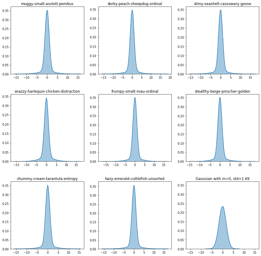
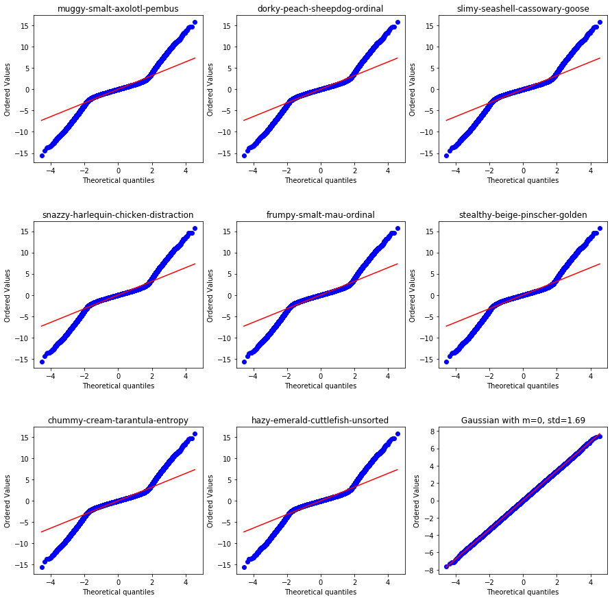
正規な分布でないことが分かっていただけたと思います。
ただ、部分的には正規分布に似た特徴が見えるので、おそらく正規分布と何かを混ぜて作ったデータでしょう。
# NORMALITY PLOTS FOR FIRST 8 VARIABLES
plt.figure(figsize=(15,15))
for i in range(8):
    plt.subplot(3,3,i+1)
    stats.probplot(train.iloc[:,1], plot=plt)
    plt.title( train.columns[i+1] )

# NORMALITY PLOT FOR GAUSSIAN
plt.subplot(3,3,9)
stats.probplot(data, plot=plt)
plt.title("Gaussian with m=0, std="+str(std))

plt.subplots_adjust(hspace=0.4)
plt.show()
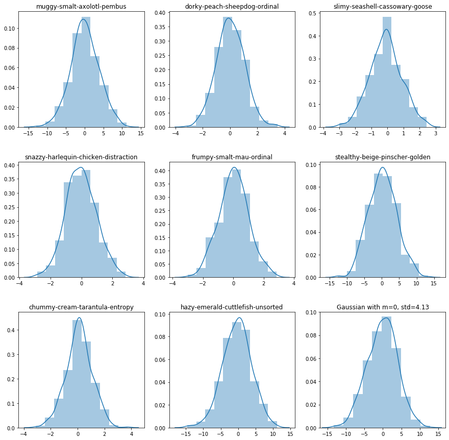
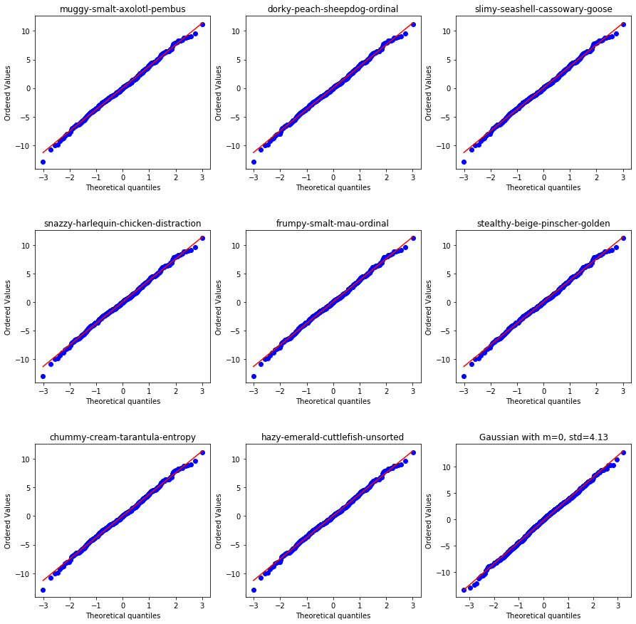
一部のデータは正規分布しています。
wheezy-copper-turtle-magicが0~511のものの中からデータを数個取ってきました。
正規分布していると直線上にplotが乗ります。
他の変数を見てみると、いくつかの変数は正規分布しているようです。
train0 = train[ train['wheezy-copper-turtle-magic']==0 ]

# PLOT FIRST 8 VARIABLES
plt.figure(figsize=(15,15))
for i in range(8):
    plt.subplot(3,3,i+1)
    #plt.hist(train0.iloc[:,i+1],bins=10)
    sns.distplot(train0.iloc[:,i+1],bins=10)
    plt.title( train.columns[i+1] )
    plt.xlabel('')

# PLOT GAUSSIAN FOR COMPARISON
plt.subplot(3,3,9)
std0 = round(np.std(train0.iloc[:,8]),2)
data0 = np.random.normal(0,std0,2*len(train0))
sns.distplot(data0,bins=10)
plt.xlim((-17,17))
plt.ylim((0,0.1))
plt.title("Gaussian with m=0, std="+str(std0))

plt.subplots_adjust(hspace=0.3)
plt.show()
# NORMALITY PLOTS FOR FIRST 8 VARIABLES
plt.figure(figsize=(15,15))
for i in range(8):
    plt.subplot(3,3,i+1)
    stats.probplot(train0.iloc[:,1], plot=plt)
    plt.title( train.columns[i+1] )

# NORMALITY PLOT FOR GAUSSIAN
plt.subplot(3,3,9)
stats.probplot(data0, plot=plt)
plt.title("Gaussian with m=0, std="+str(std0))

plt.subplots_adjust(hspace=0.4)
plt.show()
ここから質問コーナー
Q:カテゴリカルデータが512個あることはわかったけど、どうして512個個別を作ったら精度がよくなるってわかったの?
A:簡単なことで、一つのモデルでもやってみたし、512のモデルでもやってみた。その結果個別に分けたら精度が良かった。
512ってのは単純にカテゴリカルデータのユニークが512であっただけ。
EDAの時点でいろいろ考えるのが大事。
ターゲットと変数の関係が線形なのか非線形なのか。
ロジスティック回帰か単純ベイズかCARTかNNか。
あと変数の依存関係を見つけることも大切で、特定の変数だけでモデルを構築することもあります。
モデルを作成した後にモデルを表示してみて、変数の性質を観察することも大切です。
決定木をplotしたり、NNを逆方向に走らせたり。
Q:一つのモデルでやった場合も見てみたい。
A:別のカーネルでやる。特徴量選択で余分と判断した変数には0を代入して、単一のモデルに変形して予測したりします。
Q:グリッドサーチは?
A:グリッドサーチの結果4が最適なパラメーターだった。
Q:正規分布を含んでそうだから、rbfとか使ったら良いのでは?
A:512しかないmagic変数に対してrbfを使うと、高分散のためにオーバーフィットします。
(rbfというと動径基底関数カーネルのことだと思う。モデル作成の時に、正規分布を仮定しておいて、分布に重みづけすることでモデルを自由度高く変化させることができる。)
以上
第三回へつづく