With friends like these...
C-o-rr-a-ll-i-n-g d-i-tt-o-e-d l-e-tt-e-r-s
I was going to focus this week on the first task of the 20th Weekly Challenge...but what can I say? The task was a break a string specified on the command-line into runs of identical characters:
    "toolless"        →   t  oo  ll  e  ss
    "subbookkeeper"   →   s  u  bb  oo  kk  ee  p  e  r
    "committee"       →   c  o  mm  i  tt  ee
But that’s utterly trivial in Raku:
    use v6.d;

    sub MAIN (\str) {
        .say for str.comb: /(.) $0*/
    }
And almost as easy in Perl:
use v5.30;
my $str = $ARGV[0]
// die "Usage:\n $0 <str>\n";
say $& while $str =~ /(.) \1*/gx;
In both cases, the regex simply matches any character ((.)) and then rematches exactly
the same character ($0 or \1) zero-or-more times (*). Both match operations (str.comb
and $str =~) produce a list of the matched strings, each of which we then output
(.say for... or say $& while...).
As there’s not much more to say in either case, I instead turned my attention to the second task: to locate and print the first pair of amicable numbers.
The friend of my friend is my enemy
Amicable numbers are pairs of integers, each of which has a set of proper divisors
(i.e. every smaller number by which it is evenly divisible) that happen to add up to
the other number.
For example, the number 1184 is divisible by 1, 2, 4, 8, 16, 32, 37, 74, 148, 296, and 592; and the sum of 1+2+4+8+16+32+37+74+148+296+592 is 1210. Meanwhile, the number 1210 is divisible by 1, 2, 5, 10, 11, 22, 55, 110, 121, 242, and 605; and the sum of 1+2+5+10+11+22+55+110+121+242+605 is...you guessed it...1184.
Such pairs of numbers are uncommon. There are only five among the first 10 thousand integers, only thirteen below 100 thousand, only forty-one under 1 million. And the further we go, the scarcer they become: there only 7554 such pairs less than 1 trillion. Asymptotically, their average density amongst the positive integers converges on zero.
There is no known universal formula for finding amicable numbers, though the 9th century Islamic scholar ثابت بن قره did discover a partial formula, which Euler (of course!) subsequently improved upon 900 years later.
So they’re rare, and they’re unpredictable...but they’re not especially hard to find.
In number theory, the function giving the sum of all proper divisors of N
(known as the “restricted divisor function”) is denoted by 𝑠(N):
sub 𝑠 (\N) { sum divisors(N) :proper }
That trailing :proper is an “adverbial modifier” being applied to the call to divisors(N),
telling the function to return only proper divisors (i.e. to exclude N itself from the list).
And, yeah, that’s a Unicode italic 𝑠 we’re using as the function name. Because we can.
Once we have the restricted divisor function defined, we could simply iterate through each integer i from 1 to infinity, finding 𝑠(i), then checking to see if the sum-of-divisors of that number (i.e. 𝑠(𝑠(i)) ) is identical to the original number. If we only need to find the first pair of amicable numbers, that’s just:
for 1..∞ -> \number {
my \friend = 𝑠(number);
say (number, friend) and exit
if number != friend && 𝑠(friend) == number;
}
Which outputs:
(220, 284)
But why stop at one result? When it’s no harder to find all the amicable numbers:
for 1..∞ -> \number {
my \friend = 𝑠(number);
say (number, friend)
if number < friend && 𝑠(friend) == number;
}
Note that, because the amicable relationship between numbers is (by definition) symmetrical,
we changed the number != friend test to number < friend
...to prevent the loop from printing each pair twice:
(220, 284)
(284, 220)
(1184 1210)
(1210 1184)
(2620 2924)
(2924 2620)
(et cetera)
(cetera et)
The missing built-in
That would be the end of this story, except for one small problem: somewhat surprisingly,
Raku doesn’t have the divisors builtin we need to implement the 𝑠 function. So we’re
going to have to build one ourselves. In fact, we’re going to build quite a few of them...
The divisors of a whole number are all the integers by which it can be divided leaving no remainder. This includes the number itself, and the integer 1. The “proper divisors” of a number are all of its divisors except itself. The “non-trivial divisors” of a number are all of its divisors except itself or 1. That is:
    say divisors(12);                # (1 2 3 4 5 6 12)
    say divisors(12) :proper;        # (1 2 3 4 5 6)
    say divisors(12) :non-trivial;   #   (2 3 4 5 6)
The second and third alternatives above, with the funky adverbial modifiers,
are really just
syntactic honey
for a normal call to divisors but with an additional named argument:
    say divisors(12);                # (1 2 3 4 5 6 12)
    say divisors(12, :proper);       # (1 2 3 4 5 6)
    say divisors(12, :non-trivial);  #   (2 3 4 5 6)
In Raku it’s easiest to implement those kinds of “adverbed” functions using multiple dispatch, where each special case has a unique required named argument:
multi divisors (\N, :$proper!) { divisors(N).grep(1..^N) }
multi divisors (\N, :$non-trivial!) { divisors(N).grep(1^..^N) }
Within the body of each of these special cases of divisors, we just call the regular variant
of the function (i.e. divisors(N)) and then grep out the unwanted endpoint(s).
The ..^ operator generates a range
that excludes its own upper limit,
while the ^..^ operator generates a range that excludes both its bounds.
(Yes, there’s also a ^.. variant to exclude just the lower bound).
So, when the :proper option is specified, we filter the full list returned by divisors(N)
to omit the number itself (.grep(1..^N). Likewise, we exclude both extremal values when the
:non-trivial option is included (.grep(1^..^N).
But what about the original unfiltered list of divisors?
How do we get that in the first place?
The naïve way to generate the full list of divisors of a number N, known as “trial division”,
is to simply to walk through all the numbers from 1 to N, keeping all those that divide N
with no remainder...which is easy to test, as Raku has the %% is-divisible-by operator:
    multi divisors (\N) {
        # Track all divisors found so far...
        my \divisors = [];

        # For every potential divisor...
        for 1..N -> \i {
            # Skip if it's not an actual divisor...
            next unless N %% i;

            # Otherwise, add it to the list...
            divisors.push: i;
        }

        # Deliver the results...
        return divisors;
    }
Except that we’re not cave dwellers and we don't need to rub sticks together like that, nor do number theory by counting on our toes. We can get the same result far more elegantly:
multi divisors (\N) { (1..N).grep(N %% *) }
Here we simply filter the list of potential divisors (1..N), keeping only those that evenly
divide N (.grep(N %% *)). The N %% * test is a shorthand for creating a Code object
that takes one argument (represented by the *) and returns N %% that argument. In other
words, it creates a one-argument function by pre-binding the first operand of the infix
%% operator to N. If that’s a little too syntactically mellifluous for you, we could also
have written it as an explicit pre-binding of
the %% operator:
(1..N).grep( &infix:<%%>.assuming(N) )
...or as a lambda:
(1..N).grep( -> \i { N %% i } )
...or as an anonymous subroutine:
(1..N).grep( sub (\i) { N %% i } )
...or as a named subroutine:
my sub divisors-of-N (\i) { N %% i }
(1..N).grep( &divisors-of-N )
Raku aims to let us express ourselves in whichever notation we find most convenient, comfortable, and comprehensible.
Getting to the root of the problem
It’s hard to imagine a simpler solution to the problem of finding divisors than:
multi divisors (\N) { (1..N).grep(N %% *) }
But it’s also hard to imagine a less efficient one. For example, in order to find the eight
divisors of the number 2001, we have to check all 2001 potential divisors, which is 99.6%
wasted effort. Even for a number like 2100—which has thirty-six
divisors—we’re still throwing away over 98% of the 1..N sequence. And the bigger the
number,
the smaller its relative number of divisors, and the longer it takes to find them.
There must be a better way.
And, of course, there is. The simplest improvement we can make was first published back in 1202 by Fibonacci in his magnum opus Liber Abbaci. We start by observing that the divisors of a number always come in complementary pairs; pairs that multiply together to produce the number itself. For example, the divisors of 99 are:
      1    3    9
     99   33   11
...while the divisors of 100 are:
      1    2    4    5   10
    100   50   25   20   10
...and the divisors of 101 are:
      1
    101
Notice that, in each case, the top row of divisors always contains “small” integers no
greater than the square-root of the original number. And the bottom row consists entirely of
N divided by the corresponding top-row divisor. So we could find half the divisors by searching
the range 1..sqrt N (in just O(√N) steps), and then find the other half by subtracting each
element of that list from N (also in just O(√N) steps). In Raku that look like this:
    multi divisors (\N) {
        my \small-divisors = (1..sqrt N).grep(N %% *);
        my \big-divisors   = N «div« small-divisors;

        return unique flat small-divisors, big-divisors;
    }
The div operator is integer division, and putting the double angles around it makes it
a vector operator that divides N by each element of the list of small-divisors.
The flat is needed because the two list objects in small-divisors and
big-divisors are not automatically “flattened” into a single list in Raku.
The unique is needed because if N is a perfect square, we would otherwise get two copies of
its square-root (as in the above example of 10/10 among the divisor-pairs of 100).
Thinking big
It’s great that we were able to improve our O(N) algorithm to O(√N) so easily,
but even that only gets us so far. The performance of the divisors function up to
divisors(10⁹) is entirely acceptable at under 0.1 seconds,
but starts to fall off rapidly after that point:
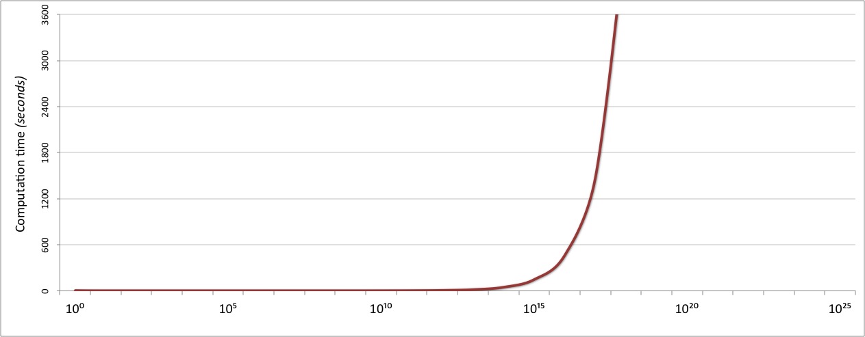
If we want our function to be usable for very large numbers, we need a better algorithm.
And, happily, the world of cryptography (which is obsessed with factoring numbers)
provides plenty of alternative techniques,
ranging from the merely very complex
to the positively eldritch.
One of the easier approaches to understand (and code!) is
Pollard’s 𝜌 algorithm,
which I explained briefly as part of a
Perl Conference keynote few years ago.
And which Stephen Schulze subsequently made available as the prime-factors function
in a Raku module named Prime::Factor.
I don’t plan to explain the 𝜌 algorithm here, or even discuss Stephen’s excellent
implementation of it...though it’s definitely worth exploring
the module’s code,
especially the sublime shortcut that uses $n gcd 6541380665835015 to instantly
detect if the number has a prime factor less than 44.
Suffice it to say that the module finds all the prime factors of very large numbers
very quickly. For example, whereas our previous implementation of divisors would take
around five seconds to find the divisors of 1 trillion, the prime-factors function finds
the prime factors of that number in less than 0.002 seconds.
The only problem is: the prime factors of a number aren’t the same as its divisors.
The divisors of 1 trillion are all the numbers by which it is evenly divisible. Namely:
1, 2, 4, 5, 8, 10, 16, 20, 25, 32, 40, 50, 64, 80, 100,
125, 128, 160, 200, 250, 256, 320, 400, 500, 512, 625,
640, 800, 1000, 1024, 1250, 1280, 1600, 2000, 2048, 2500,
[...218 more integers here...]
10000000000, 12500000000, 15625000000, 20000000000,
25000000000, 31250000000, 40000000000, 50000000000,
62500000000, 100000000000, 125000000000, 200000000000,
250000000000, 500000000000, 1000000000000
In contrast, the prime factors of a number is the unique set of (usually repeated) primes
which can be multiplied together to reconstitute the original number. For the number
1 trillion, that unique set of primes is:
2,2,2,2,2,2,2,2,2,2,2,2,5,5,5,5,5,5,5,5,5,5,5,5
...because:
2×2×2×2×2×2×2×2×2×2×2×2×5×5×5×5×5×5×5×5×5×5×5×5 → 1000000000000
To find amicable pairs we need divisors, nor prime factors. Fortunately, it’s not too hard to extract one from the other. Multiplying the complete list of prime factors produces the original number, but if we select various subsets of the prime factors instead:
                    2×2×2×2×5×5×5    → 2000
          2×2×2×2×2×2×2×2            → 256
                          2×5×5×5×5  → 1250
...then we get some of the actual divisors. And if we select the power set of the prime factors (i.e. every possible subset), then we get every possible divisor.
So all we need to do is to take the complete list of prime factors produced by
prime-factors, generate every possible combination of the elements of that list,
multiply the elements of each combination together, and keep only the unique results.
Which, in Raku, is just:
    use Prime::Factor;

    multi divisors (\N) {
        prime-factors(N).combinations».reduce( &[×] ).unique;
    }
The .combinations method produces a list of lists, where each inner list is one possible
combination of some unique subset of the original list of prime factors. Something like:
(2), (5), (2,2), (2,5), (2,2,2), (2,2,5), (2,5,5), ...
The ».reduce method call is a vector form of the
“fold” operation,
which inserts
the specified operator between every element of the list of lists on which it’s called.
In this case, we’re inserting infix multiplication via the &infix:<×> operator
...which we can abbreviate to: &[×]
So we get something like:
(2), (5), (2×2), (2×5), (2×2×2), (2×2×5), (2×5×5), ...
Then we just cull any duplicate results with a final call to .unique.
As simple as possible...but no simpler!
And then we test our shiny new prime-factor based algorithm. And weep to discover that it is catastrophically slower than our original trial division approach:
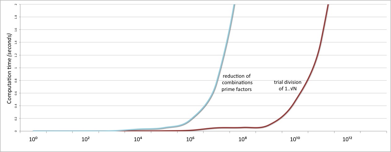
The problem here is that the use of the .combinations method is leading to a
combinatorial explosion
in some cases. We found the complete set of divisors by taking all possible
subsets of the prime factors:
    2×2×2×2×2×2×2×2×2×2×2×2×5×5×5×5×5×5×5×5×5×5×5×5 → 1000000000000
                    2×2×2×2×5×5×5                   → 2000
          2×2×2×2×2×2×2×2                           → 256
                          2×5×5×5×5                 → 1250
But that also means that we took subsets like this:
    2×2×2                                           → 8
      2×2×2                                         → 8
                      2×2×2                         → 8
    2          ×2        ×2                         → 8
In fact, we took 220 distinct 2×2×2 subsets. Not to mention 495 2×2×2×2 subsets,
792 2×2×2×2×2 subsets, and so on. In total, the 24 prime factors of 1 trillion produce
a power set of 224 distinct subsets, which we then whittle down to just 168 distinct divisors.
In other words, .combinations has to build and return a list of those 16777216 subsets,
each of which ».reduce then has to process, after which .unique immediately throws
away 99.999% of them. Clearly, we need a much better way of combining the factors
into divisors.
And, happily, there is one. We can rewrite the multiplication:
2×2×2×2×2×2×2×2×2×2×2×2×5×5×5×5×5×5×5×5×5×5×5×5 → 1000000000000
...to a much more compact:
212 × 512 → 1000000000000
We then observe that we can get all the unique subsets simply by varying the exponents of the two primes, from zero up to the maximum allowed value (12 in each case):
    2⁰×5⁰ → 1      2¹×5⁰ → 2       2²×5⁰ → 4       2³×5⁰ → 8    ⋯
    2⁰×5¹ → 5      2¹×5¹ → 10      2²×5¹ → 20      2³×5¹ → 40   ⋯
    2⁰×5² → 25     2¹×5² → 50      2²×5² → 100     2³×5² → 200  ⋯
    2⁰×5³ → 125    2¹×5³ → 250     2²×5³ → 500     2³×5³ → 1000 ⋯
    2⁰×5⁴ → 625    2¹×5⁴ → 1250    2²×5⁴ → 2500    2³×5⁴ → 5000 ⋯
    ⋮              ⋮                ⋮               ⋮            ⋱
In general, if a number has prime factors pℓ𝐼 × pmJ × pnK, then its complete set of divisors is given by pℓ(0..𝐼) × pm(0..J) × pn(0..K).
Which means we can find them like so:
multi divisors (\N) {
# Find and count prime factors of N (as before)...
my \factors = bag prime-factors(N);
# Short-cut if N is prime...
return (1,N) if factors.total == 1;
# Extract list of unique prime factors...
my \plpmpn = factors.keys xx ∞;
# Build all unique combinations of exponents...
my \ᴵᴶᴷ = [X] (0 .. .value for factors);
# Each divisor is plᴵ × pmᴶ × pnᴷ...
return ([×] .list for plpmpn «**« ᴵᴶᴷ);
}
We get the list of prime factors as in the previous version (prime-factors(N)),
but now we put them straight into a Bag data structure (bag prime-factors(N)).
A “bag” is an integer-weighted set:
a special kind of hash in which the keys are the original elements of the list
and the values are the counts of how many times each distinct value appears
(i.e. its “weight” in the list).
For example, the prime factors of 9876543210 are (2, 3, 3, 5, 17, 17, 379721).
If we put that list into a bag, we get the equivalent of:
{ 2=>1, 3=>2, 5=>1, 17=>2, 379721=>1 }
So converting the list of prime factors to a bag gives us an easy and efficient way of determining the unique primes involved, and the powers to which each prime must be raised.
However, if there is only one prime key in the resulting bag, and its corresponding count is 1,
then the original number must itself have been that prime (raised to the power of 1).
In which case, we know the divisors can only be that original number and 1,
so we can immediately return them:
return (1,N) if factors.total == 1;
The .total method simply sums up all the integer weights in the bag.
If the total is 1, there can have been only one element, with the weight 1.
Otherwise, the one or more keys of the bag (factors.keys) are the list of prime factors
of the original number (pl, pm, pn, ...), which we extract and store in an appropriate
Unicode-named variable: plpmpn. Note that we need multiple identical copies of these
prime-factor lists: one for every possible combination of exponents. As we don’t know (yet)
how many such combinations there will be, to ensure we’ll have enough we simply make the list
infinitely long: factors.keys xx ∞. In our example, that would produce the list of
factor lists like this:
((1,3,5,17,379721), (1,3,5,17,379721), (1,3,5,17,379721), ...)
To get the list of exponent sets, we need every combination of possible exponents (I,J,K,...), from zero up to the maximum count for each prime. That is, for our example:
{ 2=>1, 3=>2, 5=>1, 17=>2, 379721=>1 }
we need:
    ( (0,0,0,0,0), (0,0,0,0,1), (0,0,0,1,0), (0,0,0,1,1), (0,0,0,2,0), (0,0,0,2,1),
      (0,0,1,0,0), (0,0,1,0,1), (0,0,1,1,0), (0,0,1,1,1), (0,0,1,2,0), (0,0,1,2,1),
      (0,1,0,0,0), (0,1,0,0,1), (0,1,0,1,0), (0,1,0,1,1), (0,1,0,2,0), (0,1,0,2,1),
      (0,1,1,0,0), (0,1,1,0,1), (0,1,1,1,0), (0,1,1,1,1), (0,1,1,2,0), (0,1,1,2,1),
      (0,2,0,0,0), (0,2,0,0,1), (0,2,0,1,0), (0,2,0,1,1), (0,2,0,2,0), (0,2,0,2,1),
      (0,2,1,0,0), (0,2,1,0,1), (0,2,1,1,0), (0,2,1,1,1), (0,2,1,2,0), (0,2,1,2,1),
      (1,0,0,0,0), (1,0,0,0,1), (1,0,0,1,0), (1,0,0,1,1), (1,0,0,2,0), (1,0,0,2,1),
      (1,0,1,0,0), (1,0,1,0,1), (1,0,1,1,0), (1,0,1,1,1), (1,0,1,2,0), (1,0,1,2,1),
      (1,1,0,0,0), (1,1,0,0,1), (1,1,0,1,0), (1,1,0,1,1), (1,1,0,2,0), (1,1,0,2,1),
      (1,1,1,0,0), (1,1,1,0,1), (1,1,1,1,0), (1,1,1,1,1), (1,1,1,2,0), (1,1,1,2,1),
      (1,2,0,0,0), (1,2,0,0,1), (1,2,0,1,0), (1,2,0,1,1), (1,2,0,2,0), (1,2,0,2,1),
      (1,2,1,0,0), (1,2,1,0,1), (1,2,1,1,0), (1,2,1,1,1), (1,2,1,2,0)  (1,2,1,2,1)
    )
Or, to be express it more concisely, we need the cross-product (i.e. the X operator)
of the valid ranges of each exponent:
    #  2       3        5        17     379721
    (0..1) X (0..2) X (0..1) X (0..2) X (0..1)
The maximal exponents are just the values from the bag of prime factors (factors.values),
so we can get a list of the required exponent ranges by converting each “prime count” value
to a 0..count range: (0 .. .value for factors)
Note that, in Raku, a loop within parentheses produces a list of the final values
of each iteration of that loop. Or you can think of this construct as a
list comprehension,
as in Python: [range(0,value) for value in factors.values()] (but less prosy)
or in Haskell: [ [0..value] | value <- elems factors ] (but with less line noise).
Then we just take the resulting list of ranges and compute the n-ary cross-product
by reducing the list over the X operator: [X](0 .. .value for factors)
and store the resulting list of I,J,K exponent lists in a suitably named variable: ᴵᴶᴷ
(Yes, superscript letters are perfectly valid Unicode alphabetics, so we can certainly
use them as an identifier.)
At this point almost all the hard work is done. We have a list of the prime factors (plpmpn),
and a list of the unique combinations of exponents that will produce distinct divisors (ᴵᴶᴷ),
so all we need to do now is raise each set of numbers in the first list to the various sets
of exponents in the second list using a vector exponentiation operator (plpmpn «**« ᴵᴶᴷ)
and then multiply the list of values produced by each exponentiation ([×] .list for …)
in another list comprehension, to produce the list of divisors.
And that’s it. It’s five lines instead of one:
multi divisors (\N) {
my \factors = bag prime-factors(N);
return (1,N) if factors.total == 1;
my \plpmpn = factors.keys xx ∞;
my \ᴵᴶᴷ = [X] (0 .. .value for factors);
return ([×] .list for plpmpn «**« ᴵᴶᴷ);
}
...but with no combinatorial explosives lurking inside them. Instead of building O(2ᴺ) subsets of the factors directly, we build O(N) subsets of their respective exponents.
And then we test our shinier newer divisors implementation. And weep tears
...of relief when we find that it scales ridiculously better than the previous one.
And also vastly better than the original trial division solution:
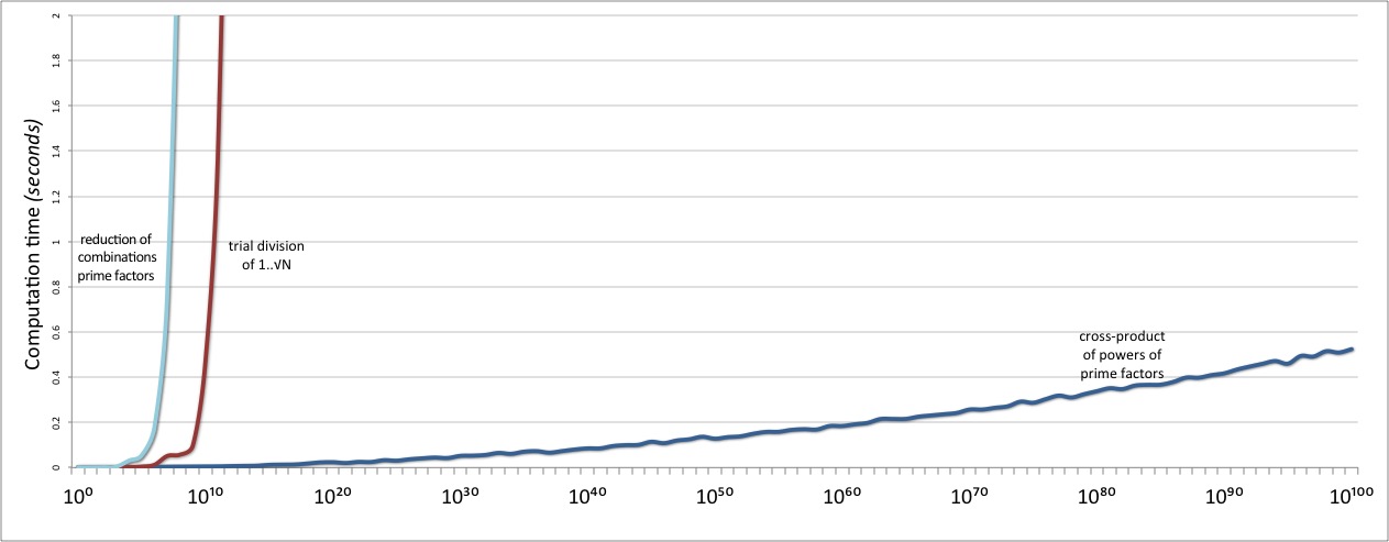
Mission accomplished!
The best of both worlds
Except that, if we zoom in on the start of the graph:
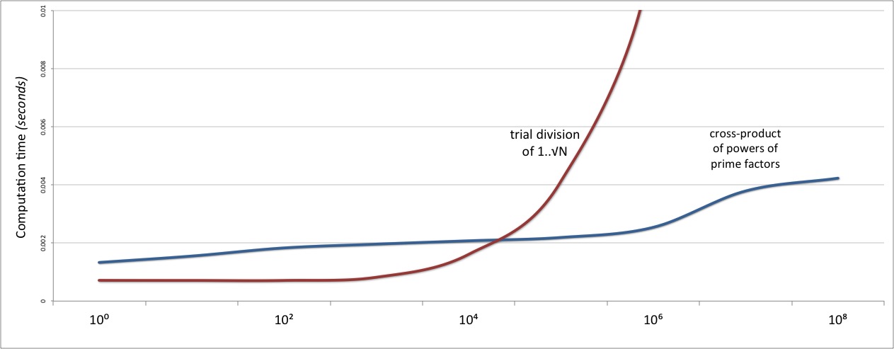
...we see that our new algorithm’s performance is only eventually better.
Due to the relatively high computational overheads of the Pollard’s 𝜌 algorithm
at its heart, and to the need to build, exponentiate, and multiply together the power set
of prime factors, the performance of this version of divisors is marginally worse
than simple trial division...at least on numbers less than N=10000.
Ideally, we could somehow employ both algorithms: use trial division for the “small” numbers,
and prime factoring for everything bigger. And that too is trivially easy in Raku.
No, not by muddling them together in some kind of Frankenstein function:
multi divisors (\N) {
if N < 10⁴ {
my \small-divisors = (1..sqrt N).grep(N %% );
my \big-divisors = N «div« small-divisors;
return unique flat small-divisors, big-divisors;
}
else {
my \factors = bag prime-factors(N);
return (1,N) if factors.total == 1;
my \plpmpn = factors.keys xx ∞;
my \ᴵᴶᴷ = [X] (0 .. .value for factors);
return ([×] .list for plpmpn «*« ᴵᴶᴷ);
}
}
Instead, we just implement both approaches independently in separate multis,
as we did previously, then modify their signatures to tell the compiler
the range of N values to which they should each be applied:
constant SMALL = 1 ..^ 10⁴;
constant BIG = 10⁴ .. ∞;
multi divisors (\N where BIG) {
my \factors = bag prime-factors(N);
return (1,N) if factors.total == 1;
my \plpmpn = factors.keys xx ∞;
my \ᴵᴶᴷ = [X] (0 .. .value for factors);
return ([×] .list for plpmpn «**« ᴵᴶᴷ);
}
multi divisors (\N where SMALL) {
my \small-divisors = (1..sqrt N).grep(N %% *);
my \big-divisors = N «div« small-divisors;
return unique flat small-divisors, big-divisors;
}
The actual improvement in this particular case is only slight; perhaps too slight to be worth the bother of maintaining two variants of the same function. But the principle being demonstrated here is important. The Raku multiple dispatch mechanism makes it very easy to inject special-case optimizations into an existing function...without making the function’s original source code any more complex, any slower, or any less maintainable.
Meanwhile, in a parallel universe...
Now that we have an efficient way to find the proper divisors of any number, we can start locating amicable pairs using the code shown earlier:
for 1..∞ -> \number {
my \friend = 𝑠(number);
say (number, friend)
if number < friend && 𝑠(friend) == number;
}
When we do, we find that the first few pairs are printed out very quickly but, after that, things start to slow down noticeably. So we might start looking for yet another way to accelerate the search.
We might, for example, notice that each iteration of the for loop is entirely independent of
any other. No outside information is required to test a particular amicable pair, and no
persistent state need be passed from iteration to iteration. And that, we would quickly
realize, means that this is a perfect opportunity to introduce a little
concurrency.
In many languages, converting our simple linear for loop into some kind of concurrent search
would require a shambling mound of extra code: to schedule, create, orchestrate, manage,
coordinate, synchronize, and terminate a collection of threads or thread objects.
In Raku, though, it just means we need to add a single five-letter modifier
to our existing for loop:
hyper for 1..∞ -> \number {
my \friend = 𝑠(number);
say (number, friend)
if number < friend &&
𝑠(friend) == number;
}
The hyper prefix tells the compiler that this particular for loop does not need to iterate
sequentially; that each of its iterations can be executed with whatever degree of concurrency
the compiler deems appropriate (by default, in four parallel threads, though there are
extra parameters
that allow you to tune the degree of concurrency to match the capacities of your hardware).
The hyper prefix is really just a shorthand for adding a call to the
.hyper method to the list being iterated.
That method converts the iterator of the object to one that can iterate concurrently.
So we could also write our concurrent loop like this:
for (1..∞).hyper -> \number {
my \friend = 𝑠(number);
say (number, friend)
if number < friend &&
𝑠(friend) == number;
}
Note that, whichever way we write this parallel for loop, with multiple iterations happening
in parallel, the results are no longer guaranteed to be printed out in strictly increasing
order. In practice, however, the low density of amicable pairs amongst the integers makes this
extremely likely anyway.
When we convert the previous for loop to a hyper for, the performance of the loop doubles.
For example, the regular loop can find every amicable pair up to 1 million in a little
over an hour; the hyper loop does the same in under 25 minutes.
To infinity and beyond
Finally, having constructed and optimized all the components of our finder of lost amities,
we can begin our search in earnest. Not just for the first amicable pair, but for the first
amicable pair over one thousand, over one million, over one billion, over one trillion,
et cetera:
# Convert 1 → "10⁰", 10 → "10¹", 100 → "10²", 1000 → "10³", ...
sub order (\N where /^ 10* $/) {
10 ~ N.chars.pred.trans: '0123456789' => '⁰¹²³⁴⁵⁶⁷⁸⁹'
}
# For every power of 1000...
for 1, 10³, 10⁶ ... ∞ -> \min {
# Concurrently find the first amicable pair in that range...
for (min..∞).hyper -> \number {
my \friend = 𝑠(number);
next if number >= friend || 𝑠(friend) != number;
# Report it and go on to the next power of 1000...
say "First amicable pair over &order(min):",
"\t({number}, {friend})";
last;
}
}
Which reveals:
First amicable pair over 10⁰: (220, 284)
First amicable pair over 10³: (1184, 1210)
First amicable pair over 10⁶: (1077890, 1099390)
First amicable pair over 10⁹: (1000233608, 1001668568)
First amicable pair over 10¹²: (1000302285872, 1000452085744)
et cetera
Well, reveals them...eventually!
Damian

Really great article. Thank you, Damian.
The blog can itself be turned into e-book for future references. Even when I had these tasks in my mind, I had no clue that it could be analysed like this. This is the quality of Damian writings. A big Thank You from the team of "Perl Weekly Challenge".