はじめに

Tensorflow 2.0 Alpha上で画像認識サンプルを動作させた過程を記載します。
基本的にはこちらの公式チュートリアルの流れに沿って導入しています。

本記事は概要版となります。
詳細は最新版TensorFlow (2.0 Alpha) 画像認識編（詳細版）で紹介しています。

構成

MacBook Pro (13-inch, 2016, Two Thunderbolt 3 ports)

TensorFlowおよび各ライブラリの読み込み

Tensorflow 2.0 Alphaが導入されている前提で進めます。
未導入の方はこちらを参照してください：最新版TensorFlow (2.0 Alpha) 動作環境構築

Tensorflowおよび各ライブラリの読み込み

from __future__ import absolute_import, division, print_function, unicode_literals

# TensorFlow and tf.keras
import tensorflow as tf
from tensorflow import keras

# Helper libraries
import numpy as np
import matplotlib.pyplot as plt

print(tf.__version__)

2.0.0-alpha0と出たらOKです。

Fashion MNISTデータセットの読み込み

Fashion MNISTとは10カテゴリ計7万枚の洋服の白黒画像(28x28ピクセル)が含まれているデータセットです。

fashion_mnist = keras.datasets.fashion_mnist

(train_images, train_labels), (test_images, test_labels) = fashion_mnist.load_data()

このコマンドを入力するとダウンロードが始まります。

ラベルごとのクラス名は以下の通りです。

ラベル	クラス
0	T-shirt/top
1	Trouser
2	Pullover
3	Dress
4	Coat
5	Sandal
6	Shirt
7	Sneaker
8	Bag
9	Ankle boot

ただし、データセットにクラス名は含まれていないため、
以下のように設定してあげましょう。

class_names = ['T-shirt/top', 'Trouser', 'Pullover', 'Dress', 'Coat','Sandal', 'Shirt', 'Sneaker', 'Bag', 'Ankle boot']

データの確認

train_images.shape

(60000, 28, 28)

len(train_labels)

train_labels

array([9, 0, 0, ..., 3, 0, 5], dtype=uint8)

test_images.shape

(10000, 28, 28)

len(test_labels)

データの準備

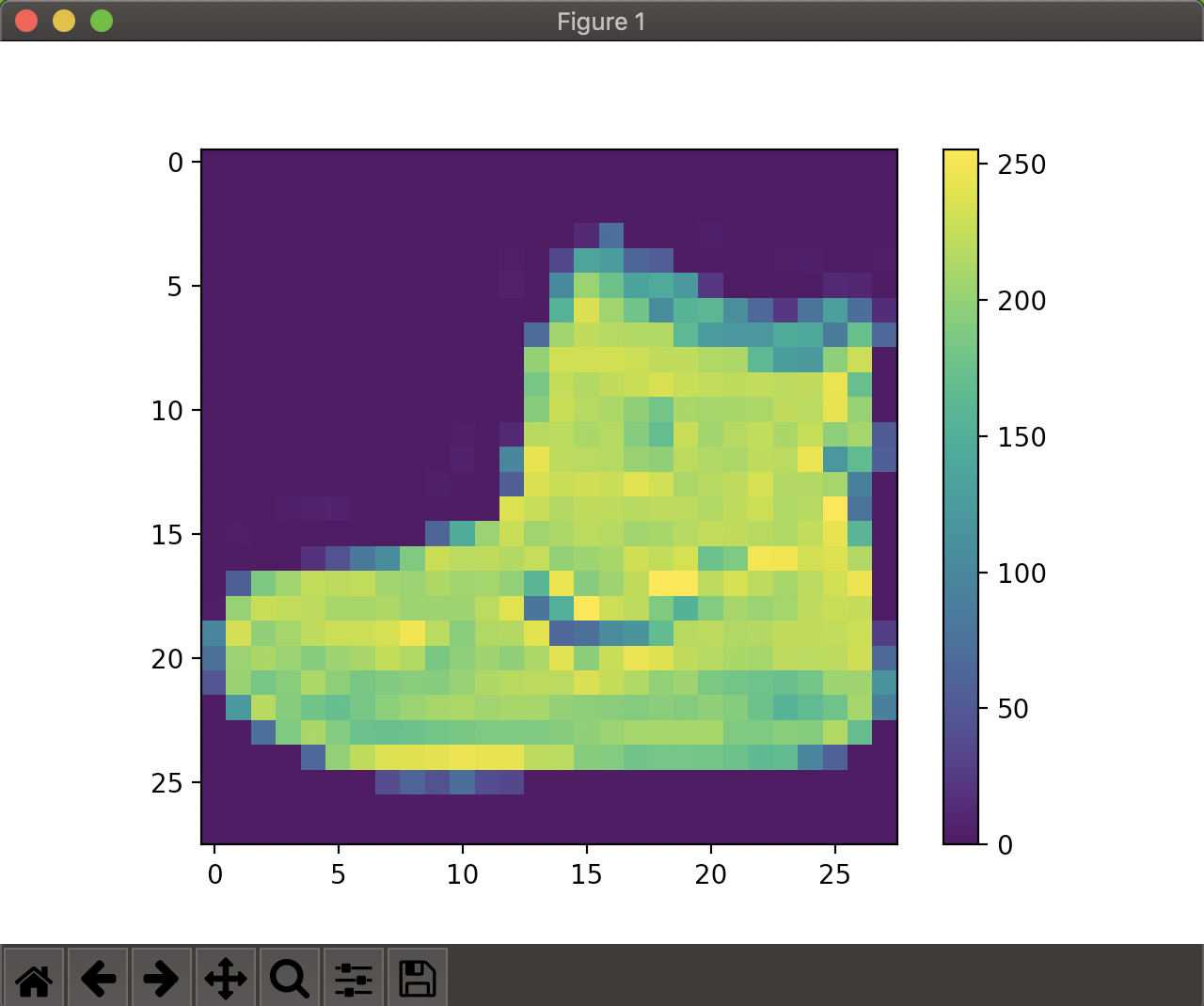
まずは画像の視覚化をしてみます。

plt.figure()
plt.imshow(train_images[0])
plt.colorbar()
plt.grid(False)
plt.show()

ウィンドウが立ち上がり、以下の画像が表示されたら成功です。

0~1の範囲にスケーリング

train_images = train_images / 255.0
test_images = test_images / 255.0

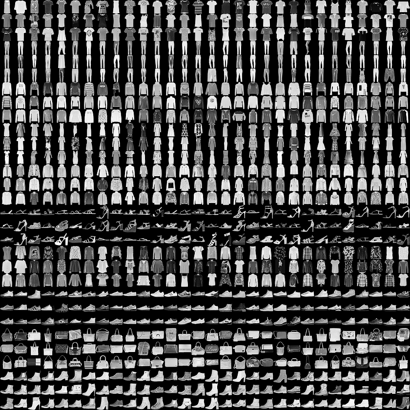
学習用セットの最初の25枚の画像を表示してみます。

plt.figure(figsize=(10,10))

for i in range(25):
    plt.subplot(5,5,i+1)
    plt.xticks([])
    plt.yticks([])
    plt.grid(False)
    plt.imshow(train_images[i], cmap=plt.cm.binary)
    plt.xlabel(class_names[train_labels[i]])

plt.show()

モデルの構築

いよいよ学習用モデルの構築に入ります。

model = keras.Sequential([
    keras.layers.Flatten(input_shape=(28, 28)),
    keras.layers.Dense(128, activation='relu'),
    keras.layers.Dense(10, activation='softmax')
])

モデルのコンパイル

ここでは以下のように設定しました。

model.compile(optimizer='adam',
              loss='sparse_categorical_crossentropy',
              metrics=['accuracy'])

モデルの学習

いよいよ学習を開始します。

以下のmodel.fitで訓練を開始します。

model.fit(train_images, train_labels, epochs=5)

Epoch 1/5
60000/60000 [==============================] - 4s 59us/sample - loss: 1.1019 - accuracy: 0.6589
Epoch 2/5
60000/60000 [==============================] - 3s 51us/sample - loss: 0.6481 - accuracy: 0.7669
Epoch 3/5
60000/60000 [==============================] - 3s 47us/sample - loss: 0.5701 - accuracy: 0.7957
Epoch 4/5
60000/60000 [==============================] - 3s 45us/sample - loss: 0.5260 - accuracy: 0.8134
Epoch 5/5
60000/60000 [==============================] - 3s 45us/sample - loss: 0.4973 - accuracy: 0.8231
<tensorflow.python.keras.callbacks.History object at 0x11d804b70>

精度としては82%程度となりました。

精度の評価

test_loss, test_acc = model.evaluate(test_images, test_labels)

print('\nTest accuracy:', test_acc)

実行結果：

Test accuracy: 0.8173

学習モデルを使った予測

学習したモデルを使ってtest_imagesの予測をしてみます。

predictions = model.predict(test_images)

最初の画像の予測結果を見てみます。

predictions[0]

array([2.2446468e-06, 7.3107621e-08, 1.1268611e-05, 1.6483513e-05,
       1.9317991e-05, 1.4457782e-01, 2.7507849e-05, 3.9779294e-01,
       6.4411242e-03, 4.5111132e-01], dtype=float32)

これは0~9のラベルに対してのそれぞれの信頼度になります。
一番信頼度が高いラベルは以下でわかります。

np.argmax(predictions[0])

続いて各信頼度をグラフ化してみましょう。

def plot_image(i, predictions_array, true_label, img):
  predictions_array, true_label, img = predictions_array[i], true_label[i], img[i]
  plt.grid(False)
  plt.xticks([])
  plt.yticks([])

  plt.imshow(img, cmap=plt.cm.binary)

  predicted_label = np.argmax(predictions_array)
  if predicted_label == true_label:
    color = 'blue'
  else:
    color = 'red'

  plt.xlabel("{} {:2.0f}% ({})".format(class_names[predicted_label],
                                100*np.max(predictions_array),
                                class_names[true_label]),
                                color=color)

def plot_value_array(i, predictions_array, true_label):
  predictions_array, true_label = predictions_array[i], true_label[i]
  plt.grid(False)
  plt.xticks([])
  plt.yticks([])
  thisplot = plt.bar(range(10), predictions_array, color="#777777")
  plt.ylim([0, 1])
  predicted_label = np.argmax(predictions_array)

  thisplot[predicted_label].set_color('red')
  thisplot[true_label].set_color('blue')

最初の画像の情報を表示してみます。

i = 0
plt.figure(figsize=(6,3))
plt.subplot(1,2,1)
plot_image(i, predictions, test_labels, test_images)
plt.subplot(1,2,2)
plot_value_array(i, predictions,  test_labels)
plt.show()

まとめ

画像認識入門編としてFashion MNISTデータセットを使ったサンプル動作を一通り実現できました。
今後は、オリジナルの学習モデルの構築を目標に勉強したいと思います。

本記事は概要版となります。
詳細は最新版TensorFlow (2.0 Alpha) 画像認識編（詳細版）で紹介しています。